DEM DSM Lidar data

Data geoportal

DEM, DSM, Lidar data

• DEM_M-34-64-D-d-1-4.asc
• DSM_M-34-64-D-d-1-4.asc

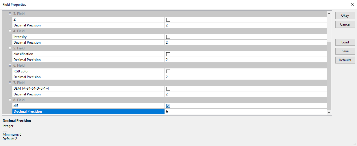
comment: save as GeoTiff, define CS, EPSG: 2180, PUWG 1992

• Lidar_M-34-64-D-d-1-4-1-3.laz

Database of topographical object BDOT10k

• 1261_SHP.zip
  • Buildings PL.PZGiK.283.1261OTBUBDA OTBUBDA

Software

• QGIS (plug-ins)
• SAGA - raster GIS software

Functionality

QGIS OpenLidarToolbox

OpenLidarToolbox - github

LiDAR Data Processing with LAStools and QGIS 3

04.01.2021 -- Pliki LAZ dostępne już dla całego zasobu

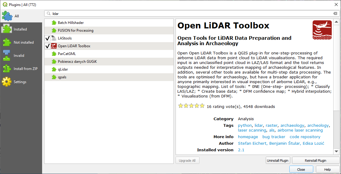
LASzip - free and lossless LiDAR compression

Before plug-in installation unzip laszip-3.4.3.tar.gz (md5) to C:/LAStools

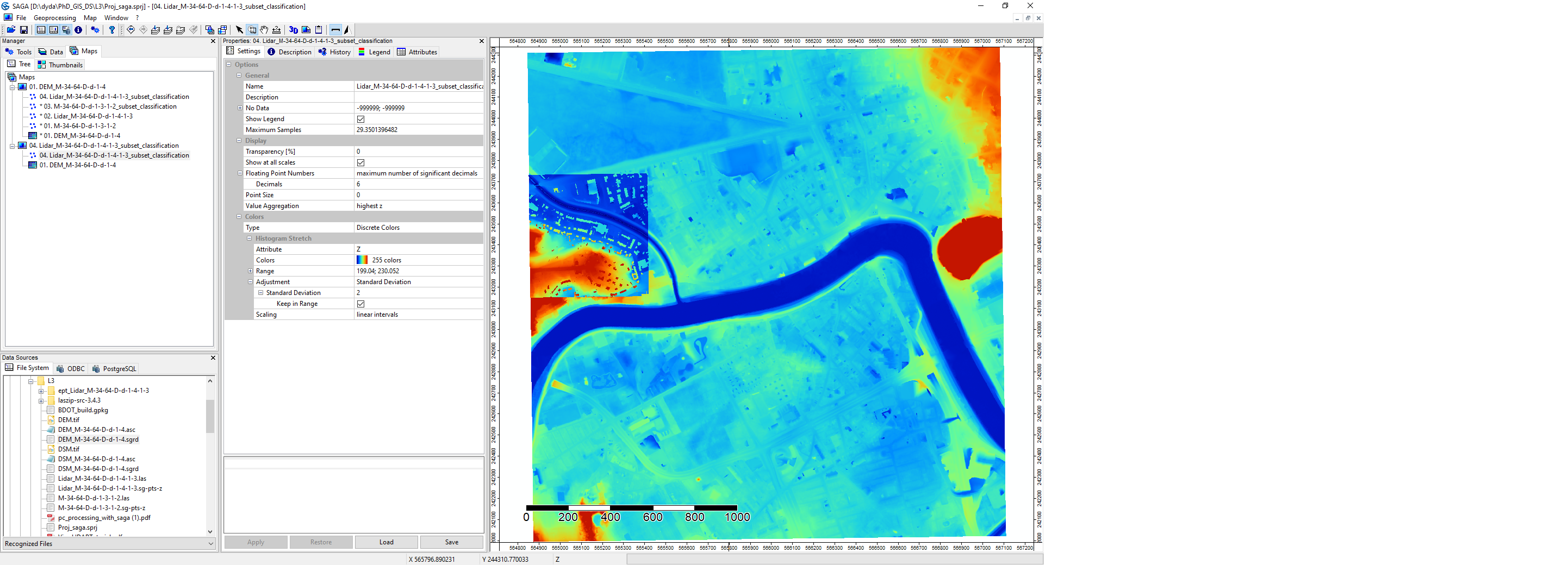
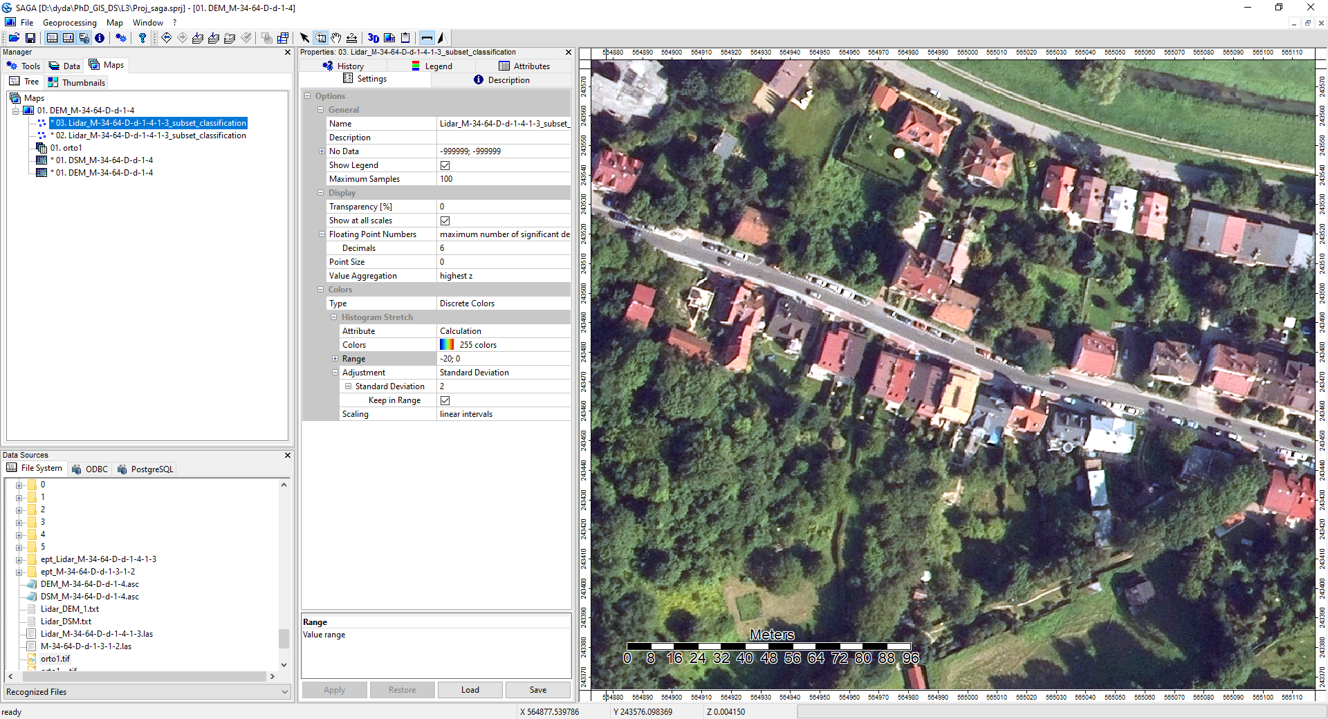
Wczytywanie chmury punktów *.LAZ

SAGA

SAGA-WIKI-Tutorials

• Tools-Import-LAS
• Shapes-Point Cloud-Point Cloud Reclassifier/Subset extractor see classes
• Tools-Import-Grids-Import Grid from ESRI asc
• Tools-Shapes-Shape-Grid Tools – Add Grid Values to Points
• Tools-Table-Field Calculatorf3-fi
• Tools-Import/Export-Shapes-Export Point Cloud to Text File

05.11.2021

DEM uncertainty

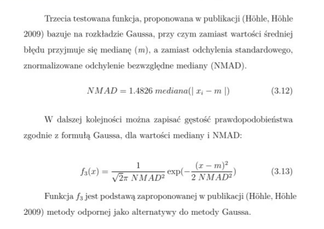
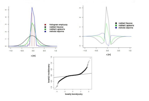
Höhle J., Höhle M., 2009 – Accuracy assessment of digital elevation models by means of robust statistical methods, ISPRS Journal of Photogrammetry and Remote Sensing 64 s. 398 - 406

Zastosowanie rozkładu Laplace’a do określania niepewności danych przestrzennych na przykładzie NMT i systemu IACS pl

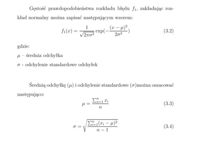
Gauss

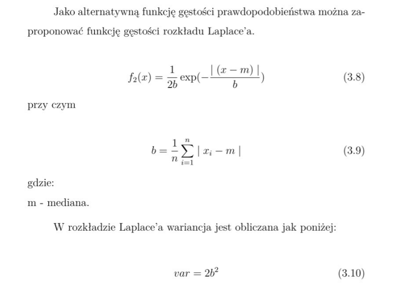
Laplace

NMAD

Data analysis OCTAVE

read1.m

clear;
plik=fopen('delta.txt'); #open file
T=fscanf(plik,'%f');  #read to matrix
fclose(plik)

--

analysis.m

T1=T([T>-99999]);
statistics(T1)
n=rows(T1)
min1=min(T1)
max1=max(T1)

me=mean(T1)
sd=std(T1)

md=median(T1)
abs1=abs(T1-md);
nmad=1.4826*median(abs1)
b=sum(abs1)/n
sd_laplace=2^0.5*b
sd_2times=1.96*sd

p1=0.975;
p2=0.95;
f1_inv=norminv(p1,me,sd)
f2_inv=norminv(p1,md,nmad)
f3_inv=md-b*sign(p1-0.5)*log(1-2*abs(p1-0.5))
percentil_975=prctile(T1,p1*100)
percentil_95=prctile(abs(T1),p2*100)

results

ans =

-2.16688000
-0.01576100
-0.00088900
 0.01364200
 2.48934900
-0.00077046
 0.03792499
 0.96825734
   163.59764549

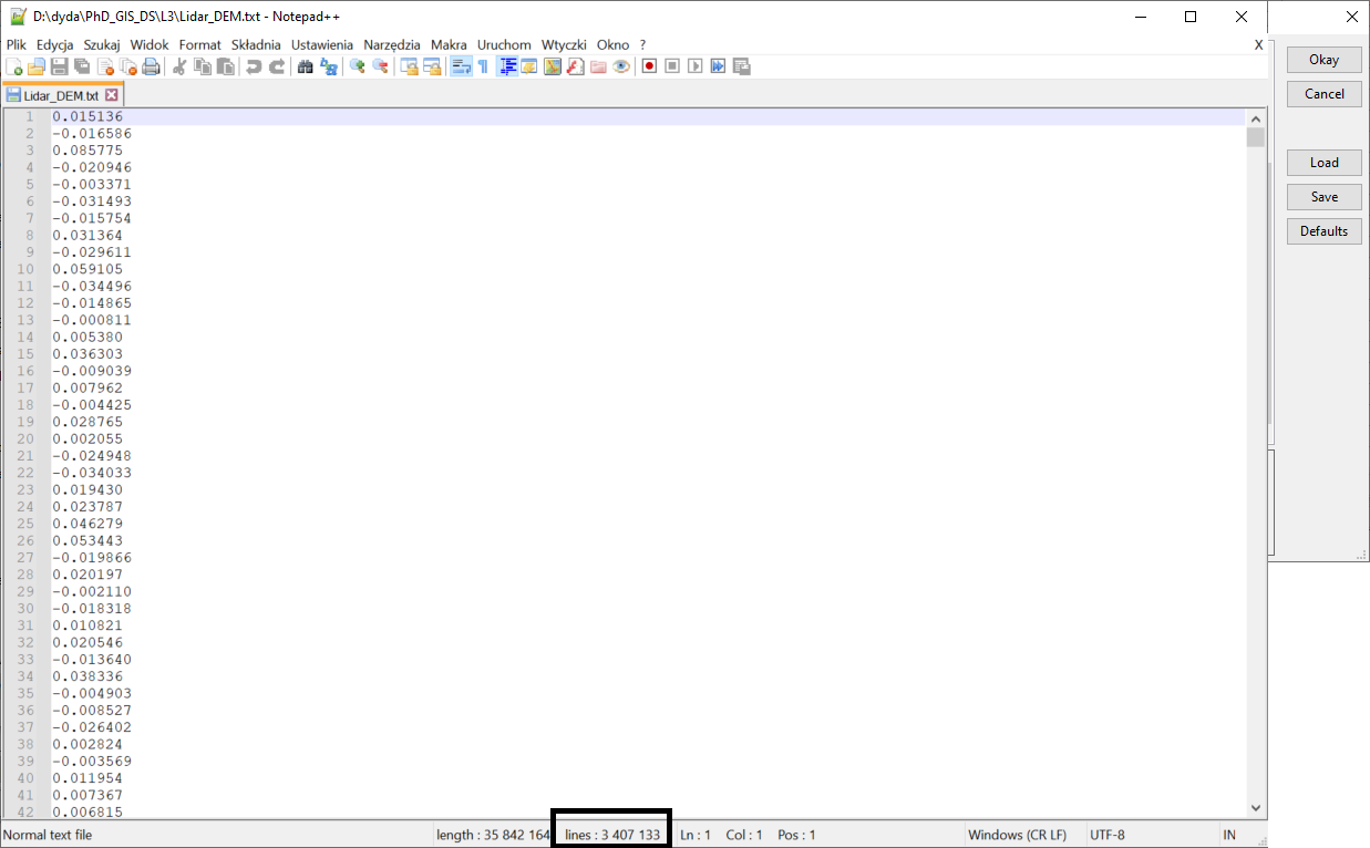
n =  3406396
min1 = -2.1669
max1 =  2.4893
me = -0.00077046
sd =  0.037925
md = -0.00088900
nmad =  0.021802
b =  0.022105
sd_laplace =  0.031262
sd_2times =  0.074333
f1_inv =  0.073561
f2_inv =  0.041841
f3_inv =  0.065332
percentil_975 =  0.064881
percentil_95 =  0.064403

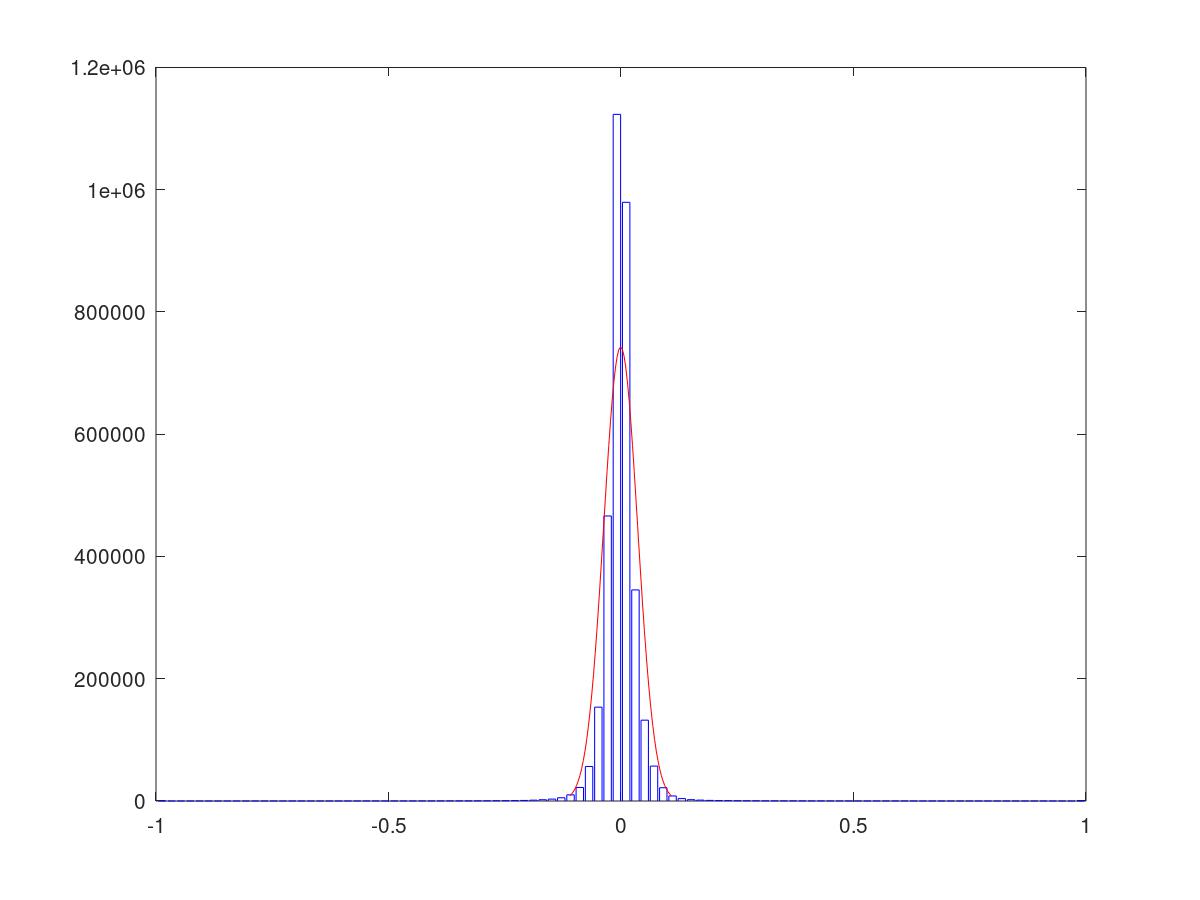
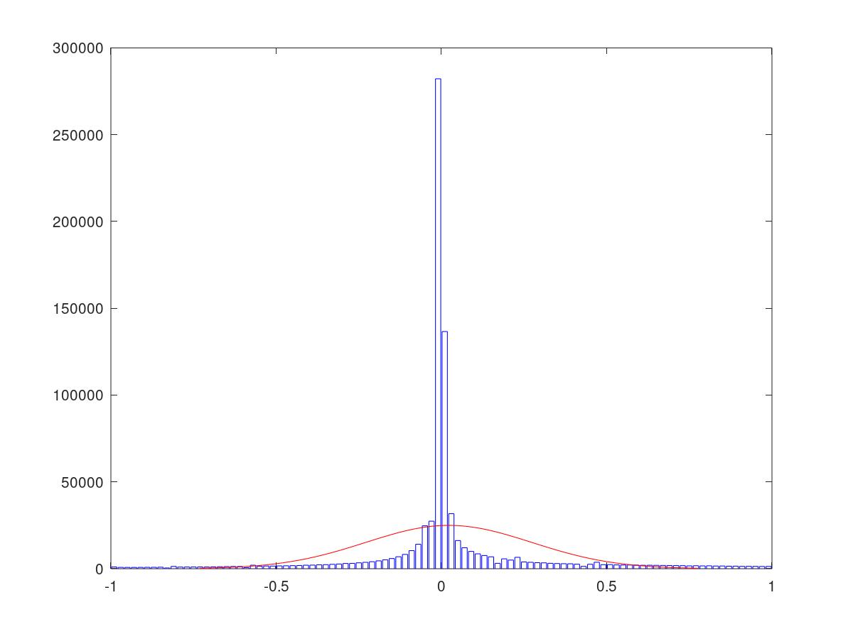
histfit

histfit(T([T>=-1 & T<=1]),100)

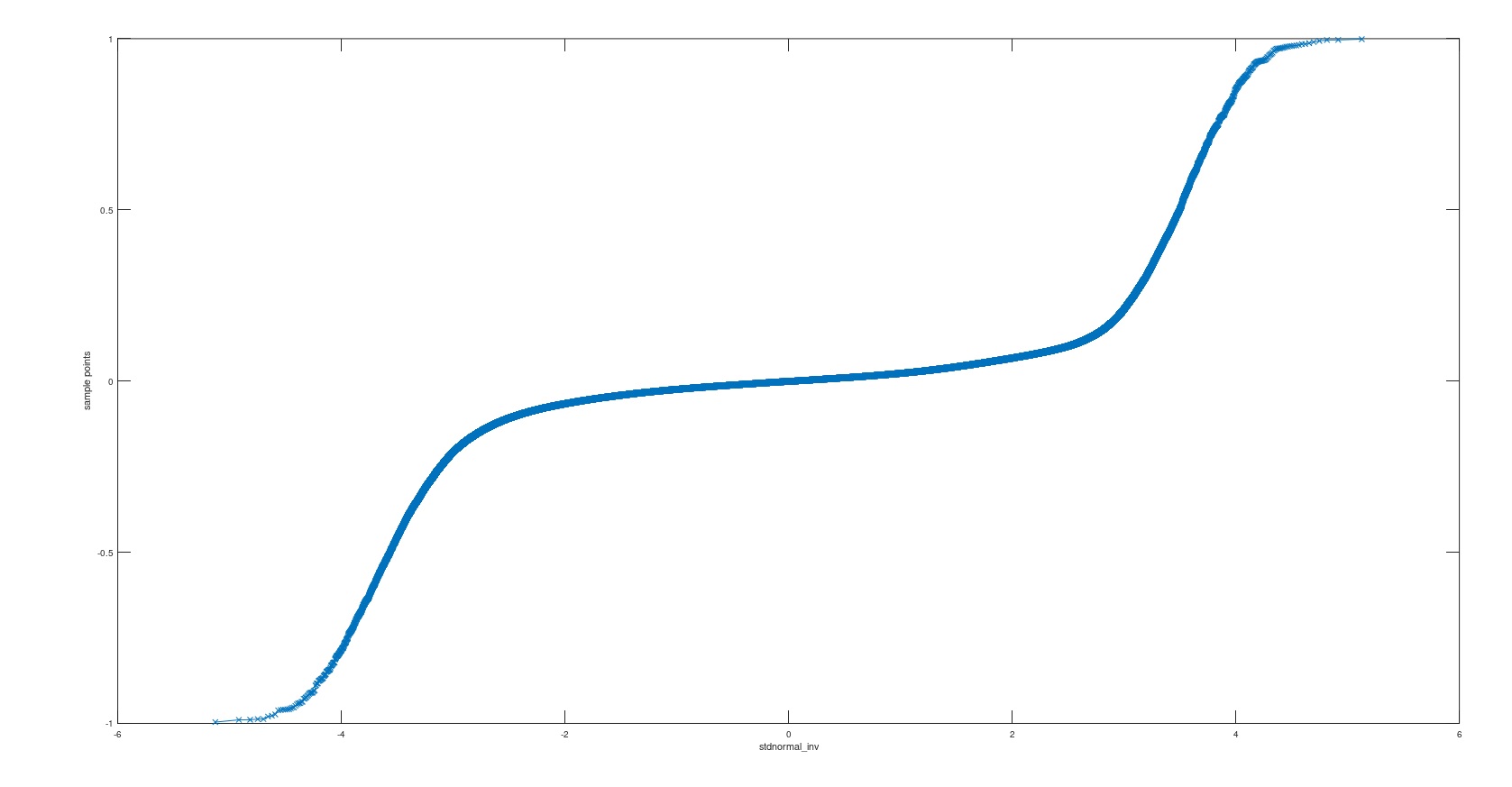
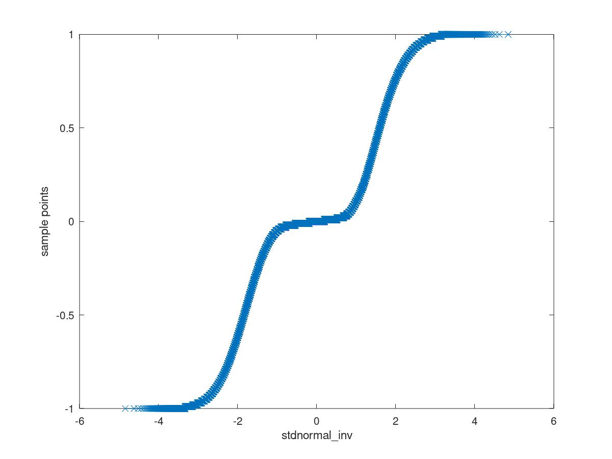
qqplot

qqplot(T([T>=-1 & T<=1]))

DEM internal uncertainty

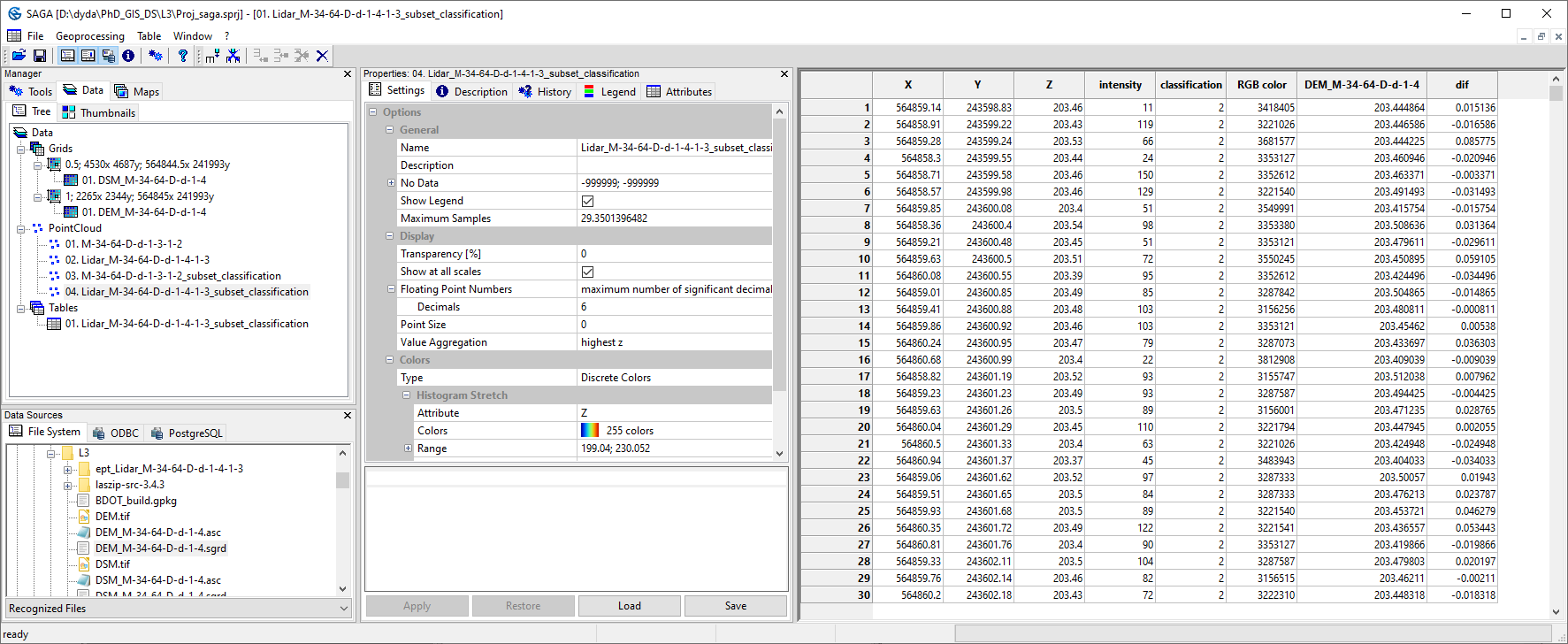
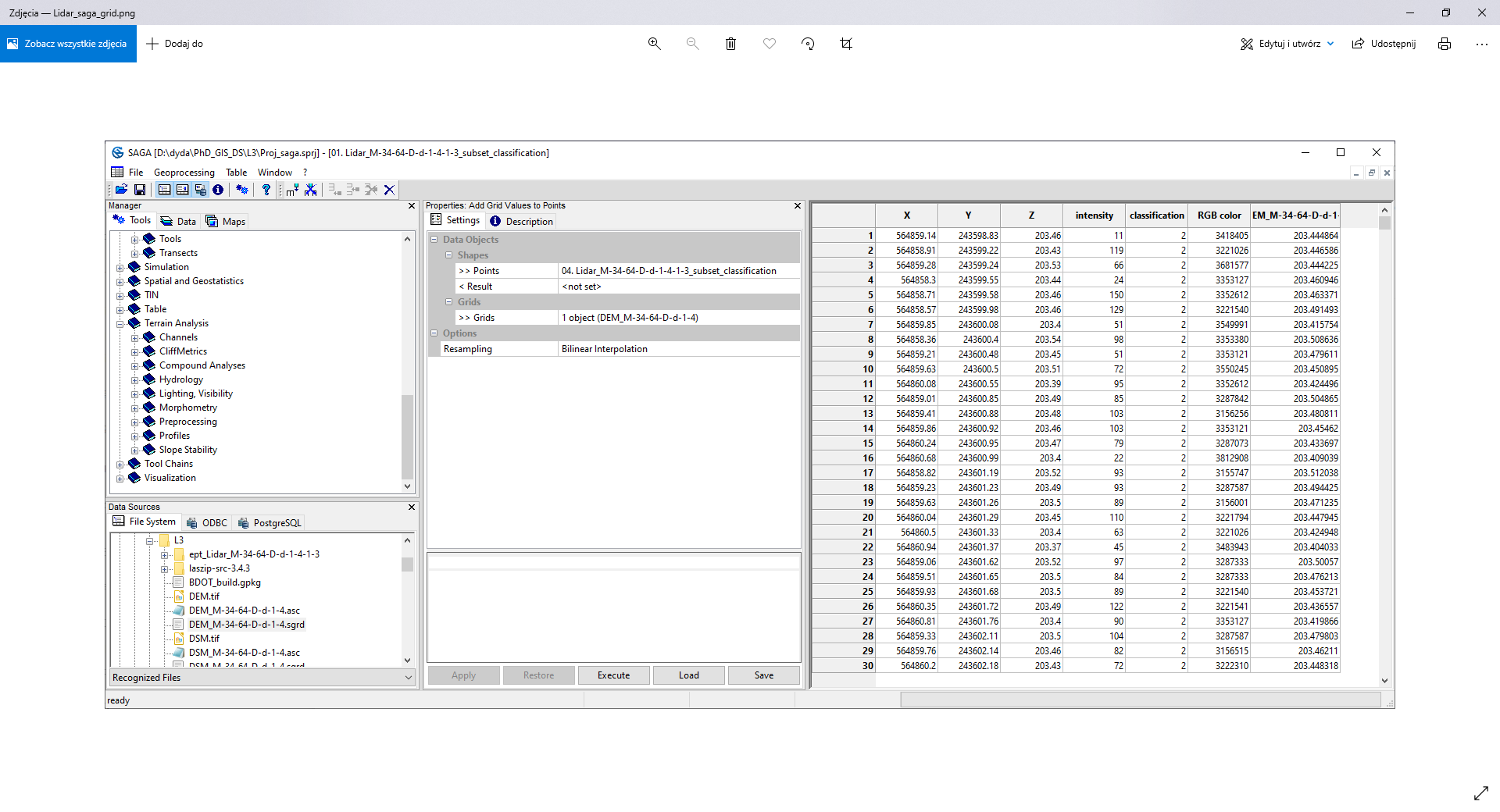
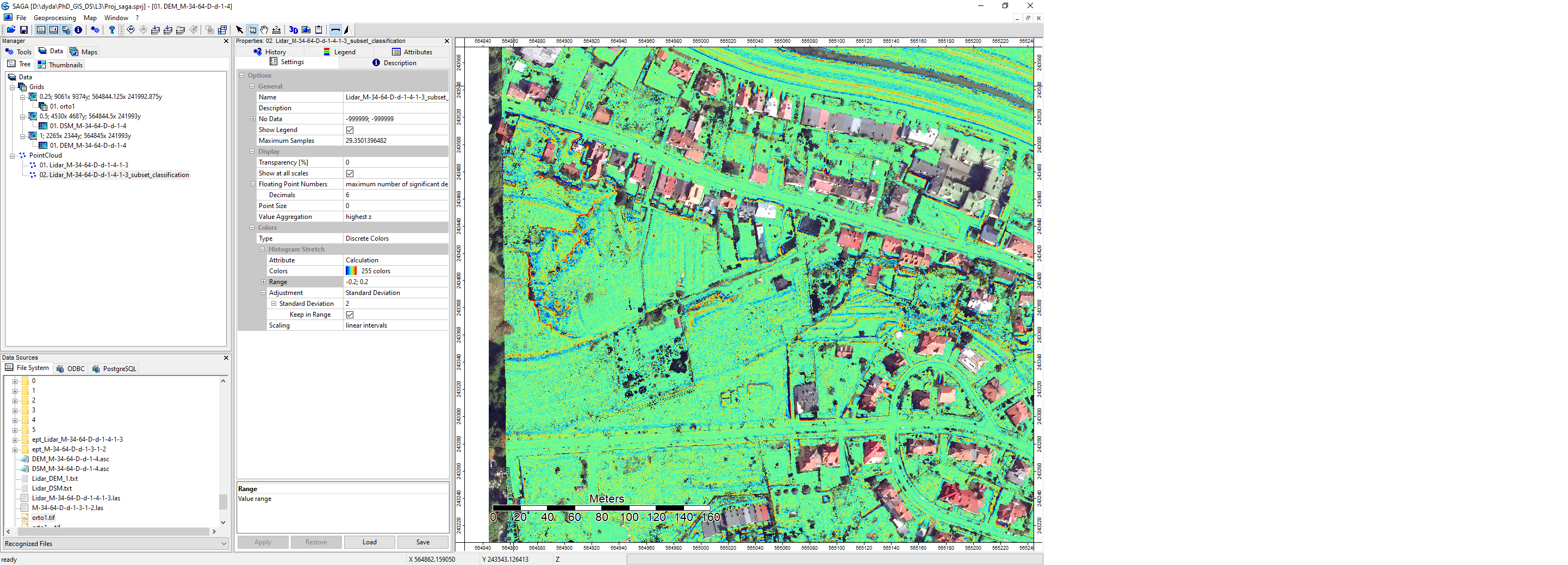
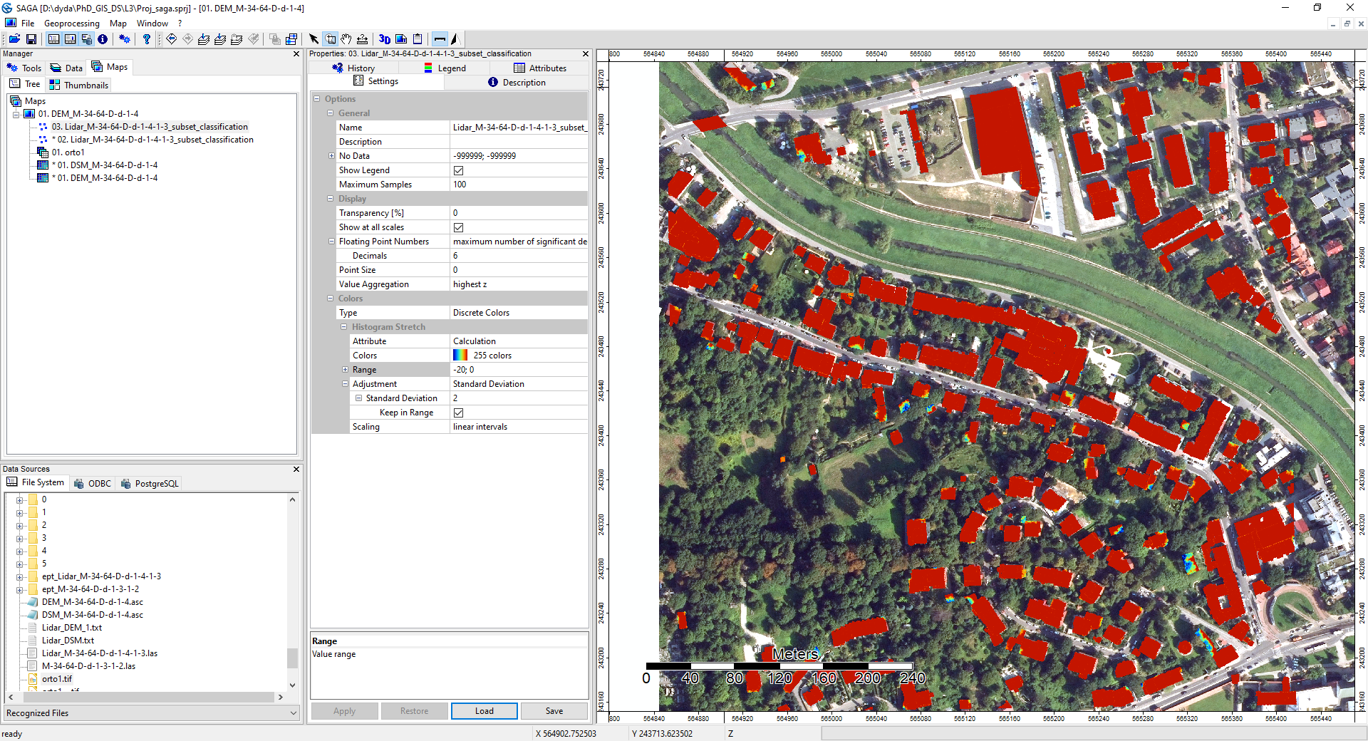
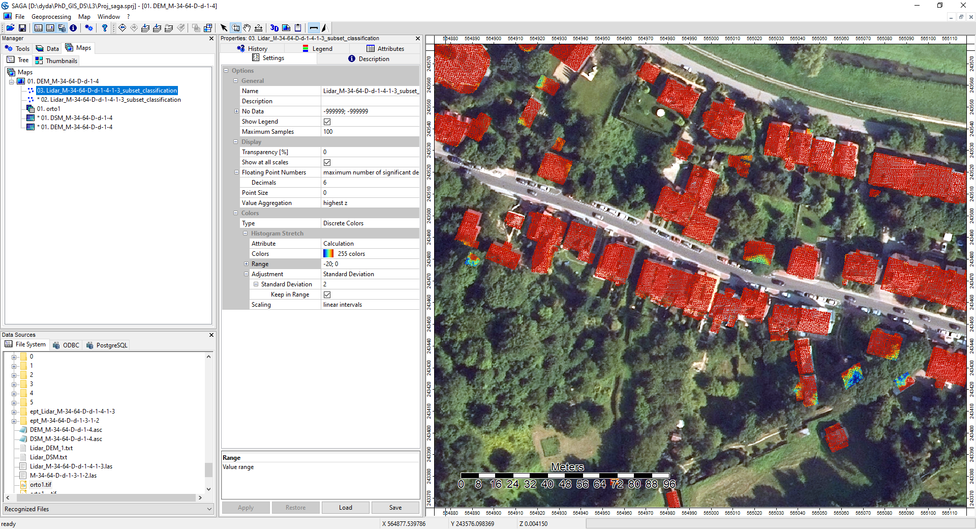
Comparison between DEM and DSM with Point Could

1. in QGIS download orto from geoportal.gov.pl using plug-in Pobieracz danych GUGIK
2. save as geotiff (right mouse klik - Export-Save, EPSG:2180)
3. Import SAGA Tools-Import/Export-Images-Import Image

4. right mouse klik Spatial Reference +proj=tmerc +lat0=0 +lon0=19 +k=0.9993 +x_0=500000 +y0=-5300000 +ellps=GRS80 +towgs84=0,0,0,0,0,0,0 +units=m +nodef

5. Check if all layers have defined CS like in point 3 : EPSG 2180, +proj=tmerc +lat0=0 +lon0=19 +k=0.9993 +x_0=500000 +y0=-5300000 +ellps=GRS80 +towgs84=0,0,0,0,0,0,0 +units=m +nodef

DEM analysis

DSM analysis

results

  -24.28000
   -0.03000
   -0.00000

    0.07000
   15.96000
   -0.10117

    2.01462
   -2.38797
   21.14126

n =  975999
min1 = -24.280
max1 =  15.960
me = -0.10117
sd =  2.0146
md = -0
nmad =  0.059304
b =  0.80173
sd_laplace =  1.1338
sd_2times =  3.9487
f1_inv =  3.8474
f2_inv =  0.11623
f3_inv =  2.4018
percentil_975 =  3.7300
percentil_95 =  4.5500

19.11.2021