ACADEMIC WEBSITE - ADRIAN HORZYK, PhD DSc

AGH University of Science and Technology in Cracow, Poland
Faculty of Electrical Engineering, Automatics, Computer Science and Biomedical Engineering
Department of Automatics and Biomedical Engineering, Field of Biocybernetics

• Didactics
• Artificial Intelligence
• Artificial Neural Networks

ARTIFICIAL NEURAL NETWORKS

Artificial neural networks are one of the most developed directions of computational intelligence and soft-computing. They are based on scientific research in field of neurobiology, neuroscience, physics, mathematics, and computer science. Neural networks are fundamental elements of brains of living creatures that enable them to reason, learn, gain knowledge, and be intelligent.

Preliminaries Brains are the only known biological “machines” that can develop intelligence and form knowledge. These biological “machines” are quite different to the computers used today, so scientists try to discover the secretes of brains in order to model artificial intelligence and knowledge for other uses than the biological ones. The first step is to discover features and functions of brain elements, especially neurons. The second step is to connect these elements to form neural networks that will be able to solve some artificial tasks. The last step is to find a way to form knowledge and create real artificial intelligence... Various kinds of artificial neural networks were developed to carry out simulations and achieve this goal. Various models of neurons were proposed. Various training strategies were constructed to adapt various kinds of these artificial neural networks to solve some given tasks and generalize them to solve also some new or similar ones.

Artificial neural networks usually work on separate samples, i.e. combinations of input data. Brains of living creatures work on sequences of continuously incoming combinations that are usually spread over time, so the previous data combinations create the context for the following associations of next input data combinations. The biological associative processes occur not only between external input data that affect the system at the same time forming various combinations but also between sequences of input data, their combinations and sequences. Automatic and active linking of data combinations and their parts (sub-combinations) is crucial for thinking, cognition and intelligent behaviors because it enables contextual recalling, generalization and creativity.

Human Brain A human brain and other parts of a human nervous system consist mainly of about: 40 000 000 000 neurons, 400 000 000 000 glial cells, 50 000 000 000 000 synaptic connections, many sense receptors of various kinds, an interneuronal space filled with cerebrospinal fluid - the medium that enables neurons to connect and interact. The human brain processes data in the quite different way than today’s computers. Inside the brain are: no compiled or interpreted programs known from today’s computers; no computer-like universal memory (RAM), no hard discs, no flash memory, no data stores or warehouses, and no relational data bases; no separated data and instructions; no separated memory and processor unit(s) alike CPU or GPU; no data tables, stacks, or lists; no computer-like instructions, conditions, (nested) loops, and equations.

Biological nervous systems can still generalize facts, rules, methods, and algorithms better than their computational counterparts. The acquired knowledge allows them to perform various intricate reasoning processes and be creative. Creativity could be more appropriate when using human-like brain structures and knowledge in a human-like manner. Human thinking is based on a nervous system and knowledge formed as consolidated associations between objects, actions, facts, rules etc. The associations can be triggered according to the context defined by a situation, previous thoughts, surroundings, needs, emotions etc. The triggered associations produce some responses that can interact with surroundings as well as broaden one’s knowledge. Moreover, the triggered associations can provide not only remembered facts and rules but also new ones according to the context of recalling that can be different from the contexts of previous training. Such behaviors are creative and occurs automatically. If creative behaviors are effective and adequate to a situation then they are intelligent; if intelligent behaviors are non-egocentric then they are wise.

Neuron What is a neuron? What features and functions does it carry out? Why do biological neurons differ in size, neurotransmitters, receptors, locations, a number of connections, and parameters of synaptic transmission? Why biological neurons relax and refract themselves? How connections are created and established? Is it a random or controlled process? How do they incorporate into the associative processes that associate data, their frequent combinations, and sequences? Is the frequency of their activations important? How do they represent data, objects, information, etc.? How do they cooperate to represent more complicated objects, tasks, sentences, rules, or algorithms? How do they represent knowledge? How do they almost immediately solve the tasks that are computationaly very complex for today’s computers? Each neuron is a living cell, so we have to consider it in its surroundings. It needs food to live and interact with other neurons, interneuronal space, glial cells, sensory cells (sensors) and actuators etc. Moreover, each body cell performs its body functions that determine its development, metabolism, energy needs, chemical ingredients and dependency on other cells. The fundamental function of neurons is to be activated for some combinations of input stimuli, and not to be activated for the others. This function makes the neuron to be a discriminator. Very important question is how does each neuron determine, which combinations should activate it, and which do not. Each neuron can be usually stimulated and activated by many various combinations of input stimuli. Such combinations can be similar as well as quite different using various subset of inputs stimulating the neuron in various moments and order.

All neurons work continuously and parallelly in time. They interract and cooperate with each other. They can be activated in different moments which determine next excitations, inhibitions, and activations. The neuronal internal states can change after external stimuli. Each neuron can be in the resting state (equilibrium potential) or in the state that reflects its recently last excitations, suppressions (inhibitions), or an activation.

Computations performed by the biological neurons are very fast, because they use knowledge that steers associations towards promising solutions based on previous experiences, learned facts and rules. Taking into account the usual frequencies of biological neuron activations (that occur between 33ms and 83ms [Longstaff]) and the usual measured intervals between presentations of various stimuli and reactions to them (usually between 300ms and 1100ms [Kalat]), we can calculate that only from 4 to 25 sequential interneuronal computational steps can be processed in a human brain. Thus, each associative reaction to presented stimuli takes constant time in a human brain. There is no place and no time for looping or searching through e.g. large data tables. Classical computer systems store various collections of data and when necessary try to search them through many times and find data that are useful for some given reasons or tasks. In the classical computer methodology hardly any task has constant computational complexity. The biological brains perform computations in a quite different way than today’s computers - they can perform various complex computations while maintaining constant computational complexity. This would not be possible without knowledge that affects and steers associative processes, and can indicate possible ways to solutions. The solutions can be found within the gained knowledge, especially due to the ability to generalize and create new variations of known objects, facts, rules, situations, processes, methods, algorithms etc. that are partially represented and associated.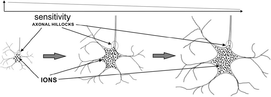

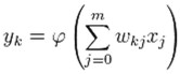
The most important aspect of the neural activity is the ability to quickly interact with other connected neurons and effectors of a neural system. Each neuron can quickly affect the other connected neurons, if it is activated; the neuron can be activated, if its internal state achieves its activation threshold. Thus, all combinations of input stimuli (which can be spread over time) that activate the neuron define the subgroup of all possible combinations which this neuron represents. The combinations of input stimuli that activate neurons usually change over time because their sizes (sensitivity) and synaptic parameters also change over time. Each neuron can represent many similar as well as differing combinations of input stimuli. All possible combinations of input stimuli that can excite or inhibit the neuron depend on the type and activities of presynaptic neurons or sense receptors. Thus, each neuron can be stimulated only by a limited subset of input combinations: the combinations that activate the neuron and the others that do not. Biological neurons rearrange these two subsets because they avoid being activated too often or too rarely. Too frequent activations of biological neurons deplete their stores of neurotransmitters, energy, and proteins and make them gather too many Ca²⁺ and Zn²⁺ ions which can lead to their death (apoptosis). Too frequent or too rare activations of neurons are not beneficial, because if a neuron represents almost all or almost no combinations it wastes the energy of its neuronal system and is functionally unuseful. Thus, neurons try to change their sensitivity to all combinations that activate them gradually growing up and raising their activation threshold. These processes automatically differentiate the sizes of neurons during their lifetime and play an important role in the further introduced associative model of neurons (as-neuron). The sizes of perikarya (somas or cell bodies) of biological neurons usually range from 4 microns (in cortical cerebellar granular layer) to 120 microns (in front motor horn cells of the spinal cord). The minimal and maximal capacities of various neurons in human nervous systems can differ even 50 thousand times, which also affect their sensitivity to input data combinations and their reactivity. This makes neurons specialize and represent only a part of all possible input data combinations.

In 1943 Warren S. McCulloch (neuroscientist) and Walter Pitts (logician) tried to understand how the brain could produce highly complex patterns by using many basic cells (neurons) that are connected together. As a result, a highly simplified model of a neuron was described in their paper "A logical calculus of the ideas immanent in nervous activity". The McCulloch-Pitts model of a neuron, which we will call an MCP neuron for short, has made an important contribution to the development of artificial neural networks - which model key basic features of biological neurons. The original MCP Neurons has many limitations. The MCP model uses a linear threshold function that provides a binary output.

In 1958 Frank Rosenblatt proposed a preceptron that developed the concept of neuron modelling. Essentially the perceptron is an MCP neuron network where the inputs are first passed through some "preprocessors," which are called association units. These association units detect the presence of certain specific features in the inputs. In fact, as the name suggests, the perceptron was intended to be a pattern recognition device, and the association units correspond to feature or pattern detectors. The perceptron is a linear classifier, i.e. a classification algorithm that makes its predictions based on a linear predictor function combining a set of weights with the feature vector. The algorithm allows for online learning, in that it processes elements in the training set one at a time.

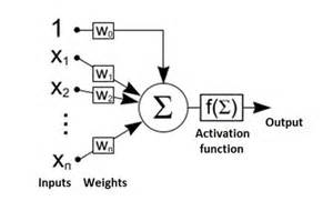
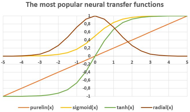
Today is mostly used the artificial neuron that receives one or more inputs (representing one or more dendrites) and sums them to produce an output (representing a biological neuron’s axon). Usually each input (signal) is weighted (multiplied by an adjustable weight value wi), and their sum is passed through a non-linear function known as an activation function, or transfer function. The transfer functions usually have a sigmoid shape, but they may also take the form of other non-linear functions, piecewise linear functions or step functions. They are also often monotonically increasing, continuous, differentiable and bounded. This model uses an extra weight (w0) that enables to add an extra value to this sum before computing the output of the transfer function. This value in the MCP neuron modelled the activation threshold of the neuron. However, the non-linear neurons do not use activation thresholds at all. The non-linear neurons work as adaptable elements that enable to approximate training data using a chosen non-linear function. This model is rather far away from the functionality of biological neurons.

For a given artificial neuron, let there be m + 1 inputs with signals x₀ through x_m and weights w₀ through w_m. Usually, the x₀ input is assigned the value +1, which makes it a bias input (threshold) with w₀ = b_k. This leaves only m actual inputs to the neuron: from x₁ to x_m.

where φ is the transfer function - description and animated presentations.

The most popular neural non-linear transfer functions are:

• linear transfer function
• sigmoid transfer function
• hyperbolic tangens transfer function
• gaussian radial transfer function

The goal of a single-layer perceptron learning algorithm is to find a separating hyperplane by minimizing the distance of misclassified points to the decision boundary. Perceptron learning cannot adapt to the data that are not linearly separable. In order to separate more complex data there are used non-linear activation funcions, more layers of an artificial neural network (ANN) and often the popular back-propagation algorithm to train such kinds of networks.

These models reduct, simplify, and even change many functions and behaviors of the biological neurons, so they are not appropriate for modelling of high-level brain functions, cognition, and intelligence.

Spiking neurons model the spiking nature of the biological neurons. The Hodgkin–Huxley spiking model can reproduce threshold–like transition between an action potential for a strong stimulus and graded response (no spike) for slightly weaker stimuli. This suggests that the emission of an action potential can be described by a threshold process. Spiking neurons "compute" when the input is encoded in temporal patterns, firing rates, firing rates and temporal corellations, and space–rate codes. An essential feature of the spiking neurons is that they can act as coincidence detectors for the incoming pulses, by detecting if they arrive in almost the same time. The leaky integrate-and-fire neuron is probably the best-known example of a formal spiking neuron model. They can either be stimulated by external current or by synaptic input from presynaptic neurons. Spiking neurons are used to construct spiking neural networks (SNN).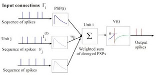

The spiking neuron models focus too much on reproducing the electrical nature of spikes, potentials, and currents of biological neurons. Unfortunately, they do not model plastic changes of biological neurons, so these model are hardly adaptable because they make changes only in synaptic weights.

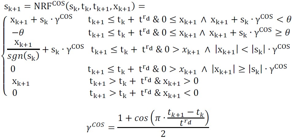
As-neurons change their excitation states in time during a relaxation or refraction process. The changes can be continuous or discrete. Both these processes restore the equilibrium state of the neuron. The relaxation process takes place if the neuron has been excited but not activated (under-threshold excitation). The refraction process takes place if the neuron has been excited and activated (over-threshold excitation). If the as-neuron is not in its equilibrium state, it temporarily stores the context of previous excitations, suppressions (inhibitions), or an activation. In such cases, its state can be easier or more difficult changed to the activation state. This temporal changes enable as-neurons to take into account previous activations of connected neurons and discriminate next excitations in their contexts. It allows to represent various sequences in the network structure constructed from as-neurons.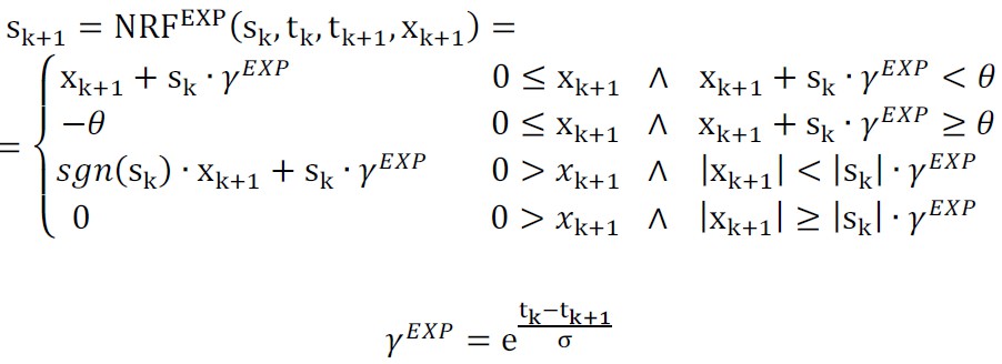

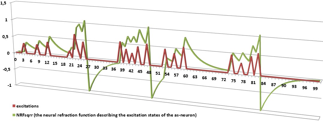
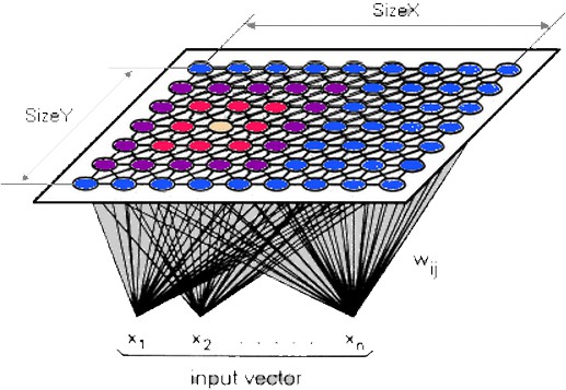
As-neurons not only model the spiking nature of the biological neurons but also various changes of their parameters and states in time. They also define the dependencies on each other. As-neurons have built-in plastic mechanisms of connecting, growing up, and optimizing their activity. It allows them to specialize in representing a special parts of the most representative input data combinations. It enables them to immediately recognize represented patterns and activate other connected neurons. This process takes constant computational time and has constant computational complexity. This recognition system does not need to search through large data tables or loop anything as is commonly used in contemporary computer science algorithms, e.g. during database processing. As-neurons can automatically connect with receptors and other as-neurons that are often activated in the same or close moments. They can also cooperate thanks to a special kind of suppressive (inhibitory) as-neurons which enable to divide the representation of input data space between cooperating as-neurons.

Moreover, each as-neuron represents every input data combination that activates it. It means, that even new combinations (that are usually similar to the trained ones) are represented by as-neurons if only they activate them. This ostensible imperfection allows them to generalize and represent classes of objects instead of the objects that have been used to adapt as-neurons. This feature automatically enables as-neurons to react to similar objects, actions, situations or in similar circumstances.

One of the most important features of as-neurons is its ability to reproduce time dependencies that take place in biological neurons and their networks. As-neurons can represent various sequences of represented objects. These sequences can represent various series of data, sentences, rules, and even algorithms. As-neurons can also recall and reproduce these sequences or produce new ones after many learned sequences. The consolidated representation and ability to represent sequences make the systems constructed from as-neurons to be creative. This feature allows to form knowledge and intelligently create new solutions that are based on previously gained knowledge.

Kohonen's SOMs are a type of unsupervised learning where neither a critic nor targer values are available. The goal is to discover some underlying classes of the data that are somehow similar. There is a topological structure imposed on the nodes in the network. A topological map is simply a mapping that preserves neighborhood relations. Nodes that are close together (directly or indirectly connected) are going to interact differently than other nodes that are far apart. Kohonen's SOMs tries to partially reproduce the connections inside the groups of cooperating neurons.

Training of SOMs:

1. Assume output nodes are connected in an array (usually 1 or 2 dimensional).
2. Assume that the network is fully connected, i.e. all nodes in input layer are connected to all nodes in output layer.
3. Randomly initialize weights with small values.
4. Use the competitive learning algorithm as follows:
   1. Randomly choose an input vector x.
   2. Determine the "winning" output node j (after the maximal output value), where wj is the weight vector connecting the inputs to output node i:
      ∀k |wj-x| ≤ |wk-x|
      
   3. Update the weights of the winning node i and alternatively also for its neighbor nodes:
      wk := wk + μ⋅χ(j,k) ⋅ (x - wk)
      where
      χ(j,k)=e(-|rk-rj|)/(2⋅σ2) is called the neighborhood function that has value 1 when j=k and falls off with the distance |rk - rj| between units j and k in the output array, μ is a learning speed coefficient. Thus, units close to the winner as well as the winner itself, have their weights updated appreciably. Weights associated with far away output nodes do not change significantly. It is here that the toplogical information is supplied. Nearby units receive similar updates and thus end up responding to nearby input patterns. The above rule drags the weight vector wi and the weights of nearby units towards the input x.

In many situations, there is less detailed information available than necessary for supervised learning. This is the role of a critic. Such kind of learning we call reinforcement learning or learinig with a critic. which can establish whether the achieved output is right or wrong.

In supervised learning we have assumed that there is given a correct target output value for each input values (usually grouped in a form a vector or a matrix). The input values together with the desired output value for them is called a training sample, training examples, or patterns. There is usually used a set of training samples (called a training set or a training data set) for adapting a chosen computational intelligence model. The example of the training samples for Iris flower classification (from ML Repository) is shown below: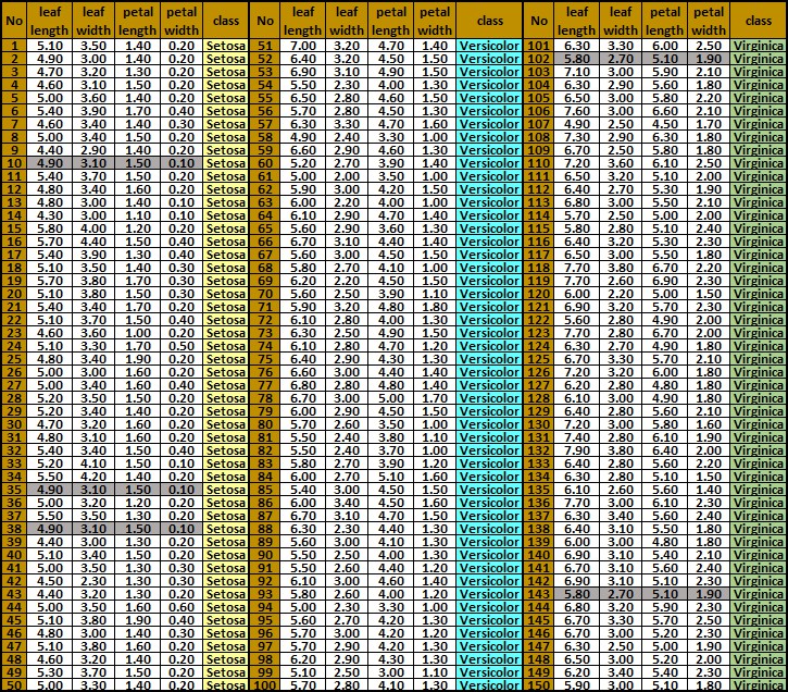

In this training data set we can distinguish:

• the input data (e.g.: 5.1, 3.5, 1.4, 0.2) and the input parameters/attributes: leaf length, leaf width, petal length and petal width
• and the target output value (e.g.: Setosa) that is here the name of the class.

Supervised learning is the process in which input data (input vectors or matrices) are one by one presented on the inputs of the chosen computational intelligence model, then the output value(s) are computed and compared to the desired output value(s). If the calculated and desired output values differ then their difference (the error value(s)) or the desired output value(s) are used to adapt the computational intelligence model and tune its internal parameters in such a way to possibly minimize the error for the next evaluations of these input data. The problem of learning is defined by competition of many training samples which we use to adapt this model and tune its internal parameters. Many times not every training sample can be satisfied and precisely represented in the trained target model. We usually define an error function for all training samples and try to minimize it during training. Its minimization is not the only goal of training because we would like to achieve the target model that will generalize training samples correctly.

Generalization is one of the major targets of machine learning that allows us to take advantages from training a chosen artificial intelligence model. Generalization is the artificial intelligence model ability to correctly evaluate new input values, which have not been used during training. By 'correctly' we mean that the difference between the calculated and desired output value(s) is acceptable. Sometimes, we do not know the desired output value(s) for new input values, but we would like to achieve the correct output value(s) that we can neither compare nor check.

We usually use various optimization methods to minimize an error function. During this process we come across many difficulties and problems:

• the problem of finding a global minimum (that is desired instead of local minima),
• the problem of overfitting (that occurs if too many free parameters of artificial intelligence models are used, which decreases the generalization ability of the model),
• the problem of input space dimensionality (known as 'curse of dimensionality'), which causes some dificulties during training if input feature vectors have very high dimension,
• the problem of possibly fast adaptation of the model in view of many competing training samples,
• the problem of contradiction, imprecission, or incorrectness of training samples (that can disable to achieve better results),
• the problem of finding an optimal structure, number of free adaptable parameters, and complexity of the model,
• the problem of extrapolation when using incorresponding function(s) (e.g. sigmoidal functions for describing periodic behaviors),
• and many others...

Gradient descent is a type of supervised learning where target output values are given in a training data set. There is used an error function that is minimized during learning using the move in the direction of decreasing gradient. This method is very simple and works as follows:

1. Choose small random initial values for the model parameters.
2. Calculate the gradient G of the error function with respect to each model parameter.
3. Change the model parameters so that we move a short distance in the direction of the greatest rate of decrease of the error, i.e., in the direction of -G.
4. Repeat steps 2 and 3 until G gets close to zero.

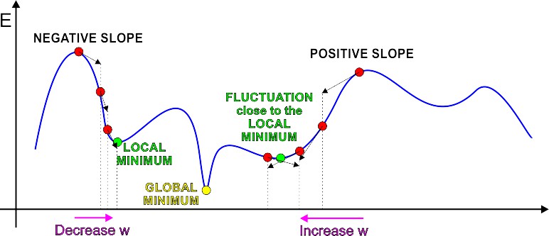
The gradient of the error function E gives us the direction in which the loss function at the current settting of the w has the steepest slope. In ordder to decrease error function E, we take a small step in the opposite direction: -G. By repeating this over and over, it moves "downhill" in E until it reaches a local minimum, where G = 0, so that no further progress is possible. Unfortunately, the reached local minimum is rarely the desired global one.

Delta rule is a gradient descent learning rule for updating the weights of the artificial neuron inputs in single-layer neural network. It is also a special case of the more general backpropagation algorithm. The delta rule is defined for a neuron j with activation function g(x) and for an input i with corresponding connection weight wji as follows:

or its simplified version for a neuron with a linear activation function:

where

• α is the learning rate (usually a small constant or a variable that can change during learning process)
• g(x) is the activation function of the neuron
• tj is the desired output value (target output)
• hj = ∑ xi wji is the weighted sum of the neuron's inputs
• yj = g(hj) is the actual computed output for the given input vector X=[x1, ..., xn]and actual weights
• xi is the i-th input (value)

The delta rule cannot be used together with perceptron step activation function because the derivative g'(hj) does not exist at zero. This rule can be derived by attempting to minimize the error in the output of the given output neuron through gradient descent. The error for the given neuron j, the calculated output value yj and the target output value tj can be measured as follows:

The delta rule can be unfortunately used to train only a single layer artificial neural networks which cannot satisfy many tasks. The discrimination property of a single layer neural network is very limited.

Back-propagation algorithm is a type of supervised learning where target output values are given in a training data set. This method also tries to minimize an error function for a given static neural network structure and training data. This method can be supported by the other methods which allow for dynamic changes in the neural network structure, e.g. genetic algorithms. 'Backpropagation' is an abbreviation for "backward propagation of errors" in MLP (multi-layer perceptron) artificial neural networks. The back propagation algorithm is a generalization of the delta rule and can be used to train multilayer neural networks thanks to the ability to propagate back the errors computed for inputs. Backpropagation requires the differentiable activation function of neurons.

We use more than one layer neural networks because a single-layer perceptrons cannot learn distinguish patterns that are not linearly separable. A multi-layer neural network can overcome this limitation and create internal representations of different features that can help to distinguish features and discriminate patterns even if they are not linearly separable.

The backpropagation learning algorithm is devided into two phases:

1. forward propagation of pattern's inputs through all neurons and all layers of the neural network till the output values of the output neurons of the network are computed,
2. update of the weights during back propagation of the computed errors on neurons' outputs.

The weights are updated using the computed output delta (error) and input activation. These two values are multiplied in order to compute the gradient for the weight correction. Next, substract a learning ratio of the gradient form the weight. The greater the learning ratio is, the faster the weights adapt, but the lower learning ratio is more accurate and limits fluctuation close to an error function minimum. The learning ratio can also change during learning process. It is usually downgraded during a training process.

The artificial neural network used for training should be constructed and its weights should be initialized by small random values. It is usually constructed from input, hidden, and output layers. There can be a few hidden layers, however there are usually used one or two such layers. The activation functions should be non-linear. On the other hand, the multi-layer neural network consisting of linear neurons could be always simplified to a single-layer neural network. There are used various logistic functions (a sigmoidal function, a tangent hyperbolic function), the softmax function, or the gaussian function. The used activation function determines the training abilities and target properties of the neural network. Artificial neurons between layers are usually fully connected (all-to-all), i.e. each neuron from one layer is connected to all neurons of the second layer.

Backpropagation training

We use a set of trainign samples sn= (x1,...,xN,t), where x1,...,xN are the inputs to the neural network and t is the desired target output. First, the network computes an output y for the given x1,...,xN which very likely differs from t since the weights are initially random. A common method for measuring the error E between the target output t and the actual output y is using the squared error measure:

Notice, that the output y depends on the weighted sum of all its inputs, where weights w_i are free parameters that enable adaptation of the neuron(s) and the network:

The backpropagation algorithm uses gradient descent to minimize error function E that is generally defined as follows:

To update the weight wi using gradient descent, the derivative of the error E with respect to the weight wi have to be computed:

If the neuron is linear then we achieve a simplified version that is exactly the delta rule for perceptron learning:

The illustration of the backpropagation algorithm

We can use stochastic, on-line, or off-line (batch) training. The on-line training makes changes to the weights immediately after the backpropagation of each training sample, while the off-line training (batch training) computes the average from all computed changes for all training samples. The stochastic training goes through the data set in a random order and updates weights immediately after each backpropagation of error to reduce its chance of getting stuck in local minima.

Artificial Associative Systems (AAS) are neural networks that are constructed from the associative neurons (as-neurons), receptors, effectors, sensorial input fields, effectorial actuators, and interneuronal space. Their way of computation is based on artificial associations that can be established and triggered. These systems allow us to use the associative model of computation that is quite different than the Turing one used in today computers and contemporary computer science. As shall be introduced in the next lecture, it can recognize already represented objects very quickly without looping any data and even without evaluating conditions. The AAS systems do not passively store data alike computer memories, but they associate data and leave them to actively interact with each other using their neural representation. They use no memory that can be used to represent whatever, but they can memorize the most representative object fetures, their sequences or classes, and facts or rules constructed from them. These systems uses active enriched AGDS structure which enables them to consolidate data representation and represent knowledge in similar form that works in living creatures. This topics will be presented in the next lecture and used to actively represent knowledge...

1. Ryszard Tadeusiewicz, Discovering neural network proprieties by means of C# programs, 2009.
2. Precise description and animated presentations of MCP model of a neuron.
3. Wulfram Gerstner and Werner M. Kistler: Spiking Neuron Models. Single Neurons, Populations, Plasticity. Cambridge Universiy Press, 2002.
4. Horzyk, A., Artificial Associative Systems and Associative Artificial Intelligence (language: Polish), Academic Publishing House EXIT, Warsaw, 2013, postdoctoral monograph, pp. 1-280.
5. Małgorzata Kossut: Synapses and Brain Plasticity., PAN
6. Kalat, J.W.: Biological grounds of of psychology. PWN, Warsaw (2006)
7. Kossut, M.: The mechanisms of brain plasticity. PWN, Warsaw (1993)
8. Longstaff, A.: Neurobiology. PWN, Warsaw (2006)