In [1]:
%plot inline -w 480 -h 480
format compact
Planowanie eksperymentu
Przykłady są dla MATLAB 2017b (jeśli funkcje są inne dla MATLAB 2014a to zaznaczono to w komentarzach)
Generowanie planu eksperymentu
Plan dwupoziomowy
In [2]:
help ff2n
 FF2N   Two-level full-factorial design.
    X = FF2N(N) creates a two-level full-factorial design, X.
    N is the number of columns of X. The number of rows is 2^N.

    Reference page in Doc Center
       doc ff2n
In [3]:
dFF2 = ff2n(2)
[s,~]=size(dFF2)
dFF2 =
     0     0
     0     1
     1     0
     1     1
s =
     4
In [4]:
dFF2 = ff2n(3)
[s,~]=size(dFF2)
dFF2 =
     0     0     0
     0     0     1
     0     1     0
     0     1     1
     1     0     0
     1     0     1
     1     1     0
     1     1     1
s =
     8
In [5]:
help fullfact
 FULLFACT Mixed-level full-factorial designs.
    DESIGN=FULLFACT(LEVELS) creates a matrix DESIGN containing the
    factor settings for a full factorial design. The vector LEVELS
    specifies the number of unique settings in each column of the design.

    Example:
        LEVELS = [2 4 3];
        DESIGN = FULLFACT(LEVELS);
    This generates a 24 run design with 2 levels in the first column,
    4 in the second column, and 3 in the third column.

    Reference page in Doc Center
       doc fullfact
In [6]:
dFF=fullfact([2 2])
dFF =
     1     1
     2     1
     1     2
     2     2
In [7]:
plot(dFF(:,1),dFF(:,2),'o')

In [8]:
dFF3=fullfact([2 2 2])
dFF3 =
     1     1     1
     2     1     1
     1     2     1
     2     2     1
     1     1     2
     2     1     2
     1     2     2
     2     2     2
In [9]:
plot3(dFF3(:,1),dFF3(:,2),dFF3(:,3),'o'), grid on
xlabel('x1'),ylabel('x2'),zlabel('x3')
view(3)

In [10]:
help fracfact
 FRACFACT Fractional factorial design for two-level factors.
    X = FRACFACT(GEN) produces the fractional factorial design defined by
    the generator string GEN.  GEN must be a sequence of "words" separated
    by spaces.  If the generator string consists of P words using K letters
    of the alphabet, then X has N=2^K rows and P columns.  Each word
    defines how the corresponding factor's levels are defined as products
    of generators from a 2^K full-factorial design.  Alternatively, GEN can
    be a cell array of strings, with one word per cell.

    [X, CONF] = FRACFACT(GEN) also returns CONF, a cell array of
    strings containing the confounding pattern for the design.

    [...] = FRACFACT(GEN, 'PARAM1',val1, 'PARAM2',val2,...) specifies one
    or more of the following name/value pairs:

        'MaxInt'      Maximum level of interaction to include in the
                      confounding output (default 2)
        'FactorNames' Cell array specifying the name for each factor
                      (default names are X1, X2, ...)

    Example:
       x = fracfact('a b c abc')

    produces an 8-run fractional factorial design for four variables, where
    the first three columns are an 8-run 2-level full factorial design for
    the first three variables, and the fourth column is the product of the
    first three columns.  The fourth column is confounded with the
    three-way interaction of the first three columns.

    See also FF2N, FULLFACT, FRACFACTGEN.

    Reference page in Doc Center
       doc fracfact
In [11]:
[dfF3,confounding] = fracfact('a b ab')
dfF3 =
    -1    -1     1
    -1     1    -1
     1    -1    -1
     1     1     1
confounding =
  7x3 cell array
    {'Term' }    {'Generator'}    {'Confounding'}
    {'X1'   }    {'a'        }    {'X1 + X2*X3' }
    {'X2'   }    {'b'        }    {'X2 + X1*X3' }
    {'X3'   }    {'ab'       }    {'X3 + X1*X2' }
    {'X1*X2'}    {'ab'       }    {'X3 + X1*X2' }
    {'X1*X3'}    {'b'        }    {'X2 + X1*X3' }
    {'X2*X3'}    {'a'        }    {'X1 + X2*X3' }
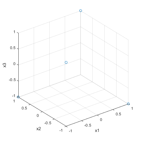
In [12]:
plot3(dfF3(:,1),dfF3(:,2),dfF3(:,3),'o'), grid on
xlabel('x1'),ylabel('x2'),zlabel('x3')
view(3)
Plan trójpoziomowy i pięciopoziomowy
In [13]:
help bbdesign
 BBDESIGN Generate Box-Behnken design.
    D=BBDESIGN(NFACTORS) generates a Box-Behnken design for NFACTORS
    factors.  The output matrix D is N-by-NFACTORS, where N is the
    number of points in the design.  Each row lists the settings for
    all factors, scaled between -1 and 1.

    D=BBDESIGN(NFACTORS,'PNAME1',pvalue1,'PNAME2',pvalue2,...)
    allows you to specify additional parameters and their values.
    Valid parameters are the following:

        Parameter    Value
        'center'     The number of center points to include.
        'blocksize'  The maximum number of points allowed in a block.

    [D,BLK]=BBDESIGN(...) requests a blocked design.  The output
    vector BLK is a vector of block numbers.

    Box and Behnken proposed designs when the number of factors was
    equal to 3-7, 9-12, or 16.  This function produces those designs.
    For other values of NFACTORS, this function produces designs
    that are constructed in a similar way, even though they were not
    tabulated by Box and Behnken and they may be too large to be
    practical.

    See also CCDESIGN, ROWEXCH, CORDEXCH.

    Reference page in Doc Center
       doc bbdesign
In [14]:
dBB = bbdesign(3)
dBB =
    -1    -1     0
    -1     1     0
     1    -1     0
     1     1     0
    -1     0    -1
    -1     0     1
     1     0    -1
     1     0     1
     0    -1    -1
     0    -1     1
     0     1    -1
     0     1     1
     0     0     0
     0     0     0
     0     0     0
In [15]:
plot3(dBB(:,1),dBB(:,2),dBB(:,3),'o')

X = [1 -1 -1 -1 1 -1 -1 -1 1 1 -1 -1;
     1 1 1 -1 1 1 1 -1 1 1 -1 -1];

Y = [-1 -1 1 -1 -1 -1 1 -1 1 -1 1 -1;
      1 -1 1 1 1 -1 1 1 1 -1 1 -1];

Z = [1 1 1 1 -1 -1 -1 -1 -1 -1 -1 -1;
     1 1 1 1 -1 -1 -1 -1 1 1 1 1];

line(X,Y,Z,'Color','k')
axis square equal

In [16]:
help ccdesign
 CCDESIGN Generate central composite design.
    D=CCDESIGN(NFACTORS) generates a central composite design for
    NFACTORS factors.  The output matrix D is N-by-NFACTORS, where N is
    the number of points in the design.  Each row represents one run of
    the design, and it has the settings of all factors for that run.
    Factor values are normalized so that the cube points take values
    between -1 and 1.

    D=CCDESIGN(NFACTORS,'PNAME1',pvalue1,'PNAME2',pvalue2,...)
    allows you to specify additional parameters and their values.
    Valid parameters are the following:

       Parameter    Value
       'center'     The number of center points to include, or 'uniform'
                    to select the number of center points to give uniform
                    precision, or 'orthogonal' (the default) to give an
                    orthogonal design.
       'fraction'   Fraction of full factorial for cube portion expressed
                    as an exponent of 1/2:  0 = whole design, 1 = 1/2
                    fraction, 2 = 1/4 fraction, etc.
       'type'       Either 'inscribed', 'circumscribed', or 'faced'.
       'blocksize'  The maximum number of points allowed in a block.

    [D,BLK]=CCDESIGN(...) requests a blocked design.  The output
    vector BLK is a vector of block numbers.  Blocks are groups of
    runs that are to be measured under similar conditions (for example,
    on the same day).  Blocked designs minimize the effect of between-
    block differences on the parameter estimates.

    See also BBDESIGN, ROWEXCH, CORDEXCH.

    Reference page in Doc Center
       doc ccdesign
In [17]:
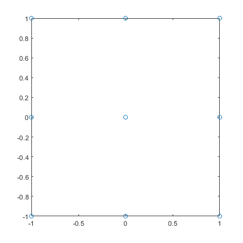
dCCD_1=ccdesign(2,'center',1, 'type','faced')
dCCD_1 =
    -1    -1
    -1     1
     1    -1
     1     1
    -1     0
     1     0
     0    -1
     0     1
     0     0
In [18]:
plot(dCCD_1(:,1),dCCD_1(:,2),'o')
In [19]:
dCCD_2=ccdesign(2,'center',1, 'type','circumscribed')
dCCD_2 =
   -1.0000   -1.0000
   -1.0000    1.0000
    1.0000   -1.0000
    1.0000    1.0000
   -1.4142         0
    1.4142         0
         0   -1.4142
         0    1.4142
         0         0
In [20]:
dCCD_3=ccdesign(2,'center',1, 'type','inscribed')
dCCD_3 =
   -0.7071   -0.7071
   -0.7071    0.7071
    0.7071   -0.7071
    0.7071    0.7071
   -1.0000         0
    1.0000         0
         0   -1.0000
         0    1.0000
         0         0
In [21]:
plot(dCCD_1(:,1),dCCD_1(:,2),'o',dCCD_2(:,1),dCCD_2(:,2),'d',dCCD_3(:,1),dCCD_3(:,2),'p')
legend('trójpoziomowy  (face-centered)', 'pięciopoziomowy - rotalny (circumscribed)','pięciopoziomowy - rotalny przeskalowany (inscribed)')

Plany równomiernie wypełniające przestrzeń
In [22]:
%plot inline -w 600 -h 600
Plan losowy o rozkładzie prawdopodobieństwa jednostajnym
In [23]:
help rand
 RAND Uniformly distributed pseudorandom numbers.
    R = RAND(N) returns an N-by-N matrix containing pseudorandom values drawn
    from the standard uniform distribution on the open interval(0,1).  RAND(M,N)
    or RAND([M,N]) returns an M-by-N matrix.  RAND(M,N,P,...) or
    RAND([M,N,P,...]) returns an M-by-N-by-P-by-... array.  RAND returns a
    scalar.  RAND(SIZE(A)) returns an array the same size as A.

    Note: The size inputs M, N, P, ... should be nonnegative integers.
    Negative integers are treated as 0.

    R = RAND(..., CLASSNAME) returns an array of uniform values of the
    specified class. CLASSNAME can be 'double' or 'single'.

    R = RAND(..., 'like', Y) returns an array of uniform values of the
    same class as Y.

    The sequence of numbers produced by RAND is determined by the settings of
    the uniform random number generator that underlies RAND, RANDI, and RANDN.
    Control that shared random number generator using RNG.

    Examples:

       Example 1: Generate values from the uniform distribution on the
       interval (a, b).
          r = a + (b-a).*rand(100,1);

       Example 2: Use the RANDI function, instead of RAND, to generate
       integer values from the uniform distribution on the set 1:100.
          r = randi(100,1,5);

       Example 3: Reset the random number generator used by RAND, RANDI, and
       RANDN to its default startup settings, so that RAND produces the same
       random numbers as if you restarted MATLAB.
          rng('default')
          rand(1,5)

       Example 4: Save the settings for the random number generator used by
       RAND, RANDI, and RANDN, generate 5 values from RAND, restore the
       settings, and repeat those values.
          s = rng
          u1 = rand(1,5)
          rng(s);
          u2 = rand(1,5) % contains exactly the same values as u1

       Example 5: Reinitialize the random number generator used by RAND,
       RANDI, and RANDN with a seed based on the current time.  RAND will
       return different values each time you do this.  NOTE: It is usually
       not necessary to do this more than once per MATLAB session.
          rng('shuffle');
          rand(1,5)

    See <a href="matlab:helpview([docroot '\techdoc\math\math.map'],'update_random_number_generator')">Replace Discouraged Syntaxes of rand and randn</a> to use RNG to replace
    RAND with the 'seed', 'state', or 'twister' inputs.

    See also RANDI, RANDN, RNG, RANDSTREAM, RANDSTREAM/RAND,
             SPRAND, SPRANDN, RANDPERM.

    Reference page in Doc Center
       doc rand

    Other functions named rand

       codistributed.rand      codistributor2dbc/rand    gpuArray.rand
       codistributor1d/rand    distributed.rand          RandStream/rand
In [24]:
RANDd=rand(10,2)
plot(RANDd(:,1),RANDd(:,2),'o'),xlabel('x1'),ylabel('x2'),grid on, grid minor
xlim([0 1]),ylim([0 1])
RANDd =
    0.8147    0.1576
    0.9058    0.9706
    0.1270    0.9572
    0.9134    0.4854
    0.6324    0.8003
    0.0975    0.1419
    0.2785    0.4218
    0.5469    0.9157
    0.9575    0.7922
    0.9649    0.9595

In [25]:
RANDd=rand(100,2);
plot(RANDd(:,1),RANDd(:,2),'o'),xlabel('x1'),ylabel('x2'),grid on, grid minor

In [26]:
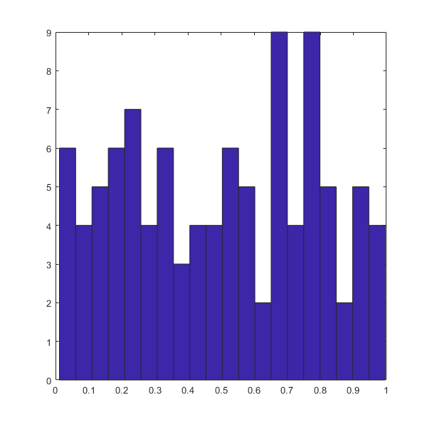
%doc cov
covM=cov(RANDd)
%doc hist
hist(RANDd(:,1),20)
covM =
    0.0803   -0.0180
   -0.0180    0.0796
Plan losowy o rozkładzie prawdopodobieństwa normalnym
In [27]:
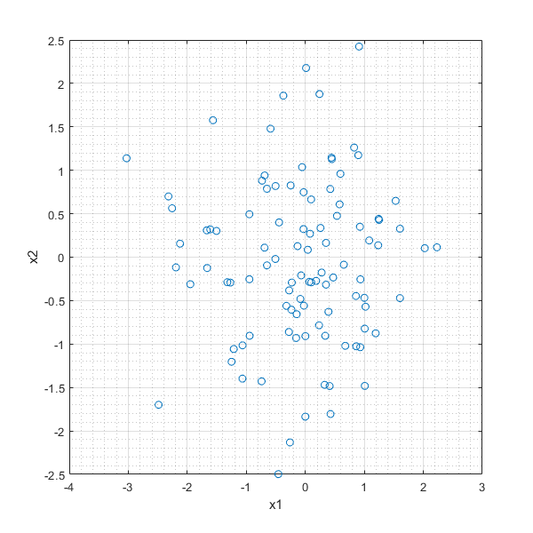
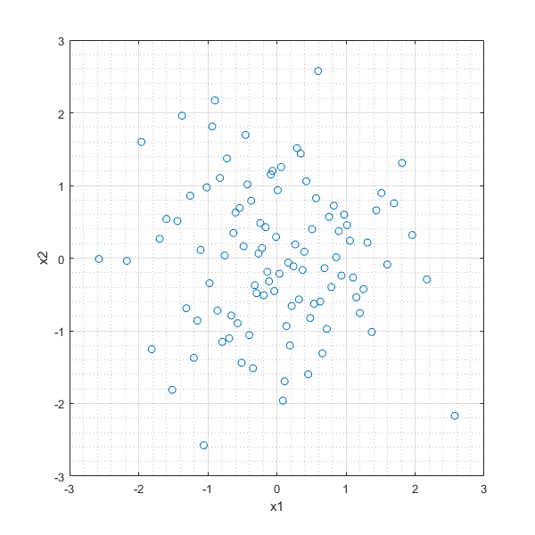
RANDNd=randn(100,2);
plot(RANDNd(:,1),RANDNd(:,2),'o'),xlabel('x1'),ylabel('x2'),grid on, grid minor
In [28]:
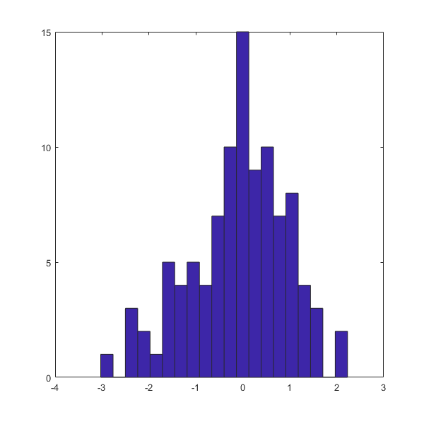
covM=cov(RANDNd)
hist(RANDNd(:,1),20)
covM =
    1.0653    0.0035
    0.0035    0.8834
Plan na podstawie wielowymiarowych sześcianów łacińskich (ang. LHS)
In [29]:
help lhsdesign
 LHSDESIGN Generate a latin hypercube sample.
    X=LHSDESIGN(N,P) generates a latin hypercube sample X containing N
    values on each of P variables.  For each column, the N values are
    randomly distributed with one from each interval (0,1/N), (1/N,2/N),
    ..., (1-1/N,1), and they are randomly permuted.

    X=LHSDESIGN(...,'PARAM1',val1,'PARAM2',val2,...) specifies parameter
    name/value pairs to control the sample generation.  Valid parameters
    are the following:

       Parameter    Value
       'smooth'     'on' (the default) to produce points as above, or
                    'off' to produces points at the midpoints of
                    the above intervals:  .5/N, 1.5/N, ..., 1-.5/N.
       'iterations' The maximum number of iterations to perform in an
                    attempt to improve the design (default=5)
       'criterion'  The criterion to use to measure design improvement,
                    chosen from 'maximin' (the default) to maximize the
                    minimum distance between points, 'correlation' to
                    reduce correlation, or 'none' to do no iteration.

    Latin hypercube designs are useful when you need a sample that is
    random but that is guaranteed to be relatively uniformly distributed
    over each dimension.

    Example:  The following commands show that the output from lhsdesign
              looks uniformly distributed in two dimensions, but too
              uniform (non-random) in each single dimension.  Repeat the
              same commands with x=rand(100,2) to see the difference.

       x = lhsdesign(100,2);
       subplot(2,2,1); plot(x(:,1), x(:,2), 'o');
       subplot(2,2,2); hist(x(:,2));
       subplot(2,2,3); hist(x(:,1));

    See also LHSNORM, UNIFRND.

    Reference page in Doc Center
       doc lhsdesign
In [30]:
LHSd=lhsdesign(10,2,'smooth','off','criterion','none','iterations',1)
plot(LHSd(:,1),LHSd(:,2),'o'),xlabel('x1'),ylabel('x2'),grid on, grid minor
LHSd =
    0.0500    0.5500
    0.2500    0.9500
    0.1500    0.2500
    0.3500    0.7500
    0.4500    0.4500
    0.7500    0.6500
    0.5500    0.8500
    0.8500    0.0500
    0.6500    0.3500
    0.9500    0.1500

In [31]:
LHSd_1=lhsdesign(10,2,'smooth','off','criterion','maximin','iterations',100)
LHSd_2=lhsdesign(10,2,'smooth','off','criterion','correlation','iterations',100)
plot(LHSd_1(:,1),LHSd_1(:,2),'o',LHSd_2(:,1),LHSd_2(:,2),'+'),xlabel('x1'),ylabel('x2'),grid on, grid minor
LHSd_1 =
    0.4500    0.8500
    0.8500    0.9500
    0.6500    0.4500
    0.5500    0.0500
    0.0500    0.1500
    0.1500    0.5500
    0.2500    0.7500
    0.7500    0.2500
    0.3500    0.3500
    0.9500    0.6500
LHSd_2 =
    0.0500    0.3500
    0.7500    0.7500
    0.6500    0.2500
    0.1500    0.9500
    0.5500    0.6500
    0.3500    0.1500
    0.8500    0.5500
    0.4500    0.8500
    0.9500    0.4500
    0.2500    0.0500

In [32]:
LHSd=lhsdesign(100,2,'smooth','off','criterion','maximin','iterations',100);
plot(LHSd(:,1),LHSd(:,2),'o'),xlabel('x1'),ylabel('x2'),grid on, grid minor

In [33]:
hist(LHSd(:,1),20)
Plan LHS o rozkładzie prawdopodobieństwa normalnym
In [34]:
mu=[0 0];       %wartość średnia
sigma=[1  0
       0  1];   %macierz kowariancji
n=100;           %liczba punktów
flag='off';      %wygładzanie
LHSNd = lhsnorm(mu,sigma,n,flag);
plot(LHSNd(:,1),LHSNd(:,2),'o'),xlabel('x1'),ylabel('x2'),grid on, grid minor
In [35]:
hist(LHSNd(:,1),20)
