Next: The Reverse Aggregation Up: Illustrative examples Previous: Illustrative examples Contents
The first problem regards finding relationships in a tree structure. This is the class C1 problem (see Section 2.2). There is a content hierarchy described as a tree, containing the set of nodes (the example is based on [16]). It is visualized in Figure 12.1.
The tree is represented by the root node: Library, and its child nodes: News, Sports, etc. The nodes are kept in the RDBMS as subject relation in the form given in Table 12.1. Parent_id and Item_id columns represent the parent-child relationship using Item_id of the node as Parent_id of its children. The root node: Library, has no real parent (it is denoted by -1 as the Parent_id value). Each node can be considered a child, as well as a parent, which implies an inherent cyclical nature of the data.
Finding all the descendants (children and children's children, and so on), or all the ascendants (parents and parents' parents, and so on) of a given node may be solved recursively. This problem is defined formally in Section 2.3.
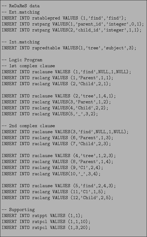
A Jelly View can be constructed which will traverse such a tree structure. The External Matching states a relationship between the Jelly View name (actually the name and arity is considered here) and the Prolog predicate which will be used as a goal to generate the contents of the view. For this purpose appropriate records in the External Matching relations have to be added (all relations mentioned below refer to Figure 11.1 and Table 11.2). Furthermore, the Internal Matching and Logic Program have to be stated. For complete SQL code refer to Figure 12.3.
The first query adds a record which establishes a relationship between the Jelly View: find and the Logic Program predicate: find (section: Ext.Matching of Figure 12.3). This predicate will be used as the goal to provide inferred records. The next two entries add information about the Jelly View attributes: their names and types. These entries will allow to create a relation which is named find and has two integer arguments: parent_id and child_id.
Next query enables access to the subject relation from the Logic Program (section Int.Matching of Figure 12.3); it establishes the Internal Matching for the Jelly View. As a result any reference to predicate tree/3, in the Logic Program, will be translated into a reference to the relation subject.
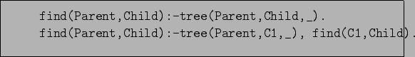
The decomposed Logic Program, which provides find predicate is added in section Logic program. The original program, in Prolog Language, is given in Figure 12.2.
The last section (Supporting) adds records creating many-to-many relationships among the External Matching, Internal Matching and Logic Program relations.
If the user issues any SQL query which addresses find Jelly View, the system takes over. It initiates the inference engine and provides inferred data. Additional arguments can be passed to the Jelly View i.e. to prevent combinatorial explosion of inferred data. The Jelly View behaves as a function which is used as a data-source (a relation). An argument is just a SQL statement which should return a single column data.
In order to find all successors of the node number 8 (for data reference see Figure 12.1 and Table 12.1) the following query should be issued (note that the restricting child_id number is given as a SQL statement: ``SELECT 8''; the reply for this query is passed to the inference engine):
     SELECT f.child_id, item_name
     FROM find('SELECT 8;',) f,
          subject s
     WHERE s.item_id=f.child_id;
And the system replies:
| child_id | item_name |
| 9 | Local |
| 10 | Collegiate |
| 11 | Professional |
| 12 | Soccer |
| 15 | Football |
| 13 | Soccer |
| 16 | Football |
| 14 | Soccer |
| 17 | Football |
The same result can be achieved issuing the following query:
     SELECT f.child_id, item_name
     FROM find(,) f, subject s
     WHERE     s.item_id=f.child_id
           AND f.parent_id=8;
The inference engine is not bounded by any arguments in this case . It generates all possible solutions and then the RDBMS selects the proper ones. Instead of 9 records, the inference engine generates 53 records. It is not a combinatorial explosion yet, however, for more complex trees definitely it will be.
Exactly the same Jelly View is capable of handling queries about the predecessors. A query: ``find all predecessors of the node number 15'' is as follows:
     SELECT *
     FROM find(,'SELECT 15;')
     ORDER BY 1;
This time the inference engine is bounded by 15 passed as the second argument to the Jelly View. It will find all predecessors of the node number 15. The system replies:
| parent_id | child_id |
| -1 | 15 |
| 1 | 15 |
| 8 | 15 |
| 9 | 15 |
As it was mentioned before, the argument of a Jelly View has to be a valid SQL SELECT statement, returning a single column. A multi row value can be used as well, for example: ``find all predecessors of nodes 10 or 4'' can be expressed as follows:
     SELECT *
     FROM find(,'SELECT 10 UNION SELECT 4;')
     ORDER BY 2,1;
And the reply is:
| parent_id | child_id |
| -1 | 4 |
| 1 | 4 |
| 2 | 4 |
| -1 | 10 |
| 1 | 10 |
| 8 | 10 |
In order to check the overall performance of the system, the same Jelly View is used to browse a larger tree structure.
The contents of the subject relation is exchanged with a new tree.
It has three children at each node and it is twelve level deep.
The number of nodes is given as a Sum of Geometric Series.
Having the following series:
To have a tree structure with three children at each node and twelve level deep, the following assumptions have to be stated:
![]() , so number of nodes in the tree is equal:
, so number of nodes in the tree is equal:
     SELECT *
     FROM find(,'SELECT max(item_id) FROM subject;')
     ORDER by 1;
The system replies:
| parent_id | child_id |
| -1 | 265719 |
| 0 | 265719 |
| 3 | 265719 |
| 12 | 265719 |
| 39 | 265719 |
| 120 | 265719 |
| 363 | 265719 |
| 1092 | 265719 |
| 3279 | 265719 |
| 9840 | 265719 |
| 29523 | 265719 |
| 88572 | 265719 |
The response is given in 13.5 seconds. Assuming that the tree structure has 265720 nodes, it is a satisfying result. The experiment was conducted using Mobile Intel Celeron CPU 1.50GHz, Linux 2.4.21, PostgreSQL 7.2.1, Unix ODBC 2.1.1, SWI-Prolog 5.0.10. The following timings have been achieved:
     real    0m13.593s
     user    0m10.140s
     sys     0m0.860s
Where real is the total execution time, user is the CPU time allocated to the process, sys is the OS overhead (interprocess communication, I/O, library calls etc.).
Furthermore:
![]() is the RDBMS overhead12.1.
is the RDBMS overhead12.1.
The database overhead becomes significant if the system generates larger amounts of records. It is expected, because the database is fed with all records generated by the inference engine. The records have to be inserted into a temporary table before the user query can be completed. So, the system throughput is limited by the RDBMS throughput.
Timings for different size of the output data are gathered in Table 12.2. In this case the query is: ``find all successors of the given node''. The given node is denoted as parent_id, the number of rows that are returned as a reply is denoted as # records. The query for the first row of the Table 12.2 is:
     SELECT *
     FROM find('SELECT 29523',)
     ;
The queries for subsequent rows in the table differ by the parent_id number in the first argument of the find Jelly View.
|
Graph traversal problems can also be easily solved. Example Prolog programs of such applications are given in [4].
Igor Wojnicki 2005-11-07
![\includegraphics[width=0.5\textwidth]{pic/tree}](img246.png)